Gauge R&R Calculator (Average & Range)
Is the measurement system good enough to trust the numbers? Enter the number of parts, appraisers and trials, plus the three summary ranges from your study, and this calculator returns the repeatability (EV), reproducibility (AV), combined gauge R&R, part variation and total variation, then reports %GRR against total variation, %P/T against the tolerance, and the number of distinct categories (ndc). It uses the Average and Range (Xbar-R) method and shows every formula and constant.
Engineering estimate, not a quote. A gauge R&R is a guideline on measurement capability, not a pass/fail stamp; the characteristic, the risk and the cost of a wrong reading decide whether a given result is good enough.
How this works
A dimensional report answers one question: does the part measure in spec? But that answer is only as good as the device and the people who took the reading. Hand the same molded part to two inspectors with two calipers and you can get two numbers; hand it to the same inspector twice and you can still get two numbers. A gauge repeatability and reproducibility study — gauge R&R for short — puts a size on that measurement noise so you know how much of the variation you are seeing is the parts and how much is the measuring. If the measurement noise is large next to the tolerance, the inspection data cannot be trusted, no matter how carefully the parts were made.
Repeatability and reproducibility. Gauge R&R splits measurement variation into two parts. Repeatability — called equipment variation, EV — is the scatter you get when one appraiser measures the same part several times with the same gauge; it is the gauge talking to itself. Reproducibility — appraiser variation, AV — is the extra scatter you get when different appraisers measure the same parts; it is operator-to-operator bias in how they seat the part, read the scale or apply probe force. The two combine in quadrature into the total gauge R&R, because they are independent sources of variance: GRR = √(EV² + AV²).
The Average and Range method. The quickest hand-checkable method, and the one this tool uses, is the Average and Range (Xbar-R) method. You run the study — typically 10 parts, 3 appraisers, 2 or 3 trials — then collapse it into three numbers. R̄ (Rbar) is the average of every appraiser-and-part range, where a range is the spread between an appraiser's repeated trials on one part; it drives repeatability. X̅diff is the difference between the highest and lowest appraiser overall averages; it drives reproducibility. Rp is the range of the ten part averages; it drives the part-to-part spread. From those:
The K constants. K1, K2 and K3 are tabulated multipliers that turn an average range into a standard deviation. They depend on the counts: K1 on trials, K2 on appraisers, K3 on parts. This tool uses the 1-sigma values — K1 = 0.8862 for 2 trials and 0.5908 for 3; K2 = 0.7071 for 2 appraisers and 0.5231 for 3; and K3 = 0.7071, 0.5231, 0.4467, 0.4030, 0.3742, 0.3534, 0.3375, 0.3249, 0.3146 for 2 through 10 parts. They are simply 1/d2 and 1/d2* from the control-chart range statistics (K1 = √π/2 = 0.8862 for two readings, for example) and are published openly in SAS/QC documentation and in vendor measurement-systems references. Older AIAG worksheets carry the same constants pre-multiplied by 5.15 sigma (4.56, 3.05; 3.65, 2.70; and so on) — the ratios %GRR and ndc come out identical, because the sigma multiplier cancels. Only %P/T, which compares to a fixed tolerance, depends on whether you spread the gauge over 6 sigma (the Minitab and modern default) or 5.15 sigma (the AIAG legacy). The tool lets you choose and always tells you which it used.
Why there are two percentages. %GRR against total variation asks whether the gauge can resolve this process — the actual spread of the parts you measured. %P/T against the tolerance asks whether the gauge is precise enough for this drawing. They can disagree sharply. A gauge can look fine against a wide total variation and still swallow a big fraction of a tight tolerance, or the reverse. Report both. And watch the trap built into %GRR: if you hand the study ten nearly identical parts, the part variation PV collapses, the gauge R&R looks enormous as a share of almost nothing, and ndc crashes — not because the gauge got worse but because the study starved it of part spread. Pick parts that span the real process range.
ndc — how many bins the gauge can see. The number of distinct categories is floor(1.41 × PV / GRR), with a floor of 1. It is the count of non-overlapping groups the measurement system can reliably tell apart across the part spread. The 1.41 is √2. An ndc of 1 means the gauge can essentially only sort pass from fail; the common guidance is that ndc should be at least 5 before you lean on the data for process control or capability (Cp/Cpk) work. ndc is always truncated down, never rounded up, so 4.9 reports as 4.
Worked examples
The calculator is checked against three cases computed by hand with the 1-sigma constants. Press Load the worked example to reproduce the first.
Case C is the one worth staring at. The same gauge reports 14.2% against total variation and 6.1% against the tolerance, because the parts in that study used only about a fifth of the allowed spec band. Neither number is wrong; they answer different questions. If you only ever quoted %P/T you would never notice that the gauge is working fairly hard to resolve the actual process.
Molded-part traps that inflate gauge R&R
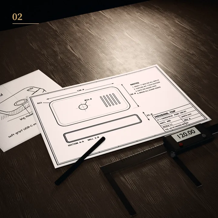
Measurement system studies on injection-molded parts have failure modes that a machined-metal study never shows. Thin walls flex under probe force, so contact gauges read differently depending on how hard the operator pushes — a classic reproducibility killer. Parting-line flash and gate vestige sit right where a caliper jaw lands, adding false size. Parts are still shrinking after ejection, so a reading taken five minutes out of the press differs from one taken the next day. Textured or matte surfaces scatter the light that optical and laser gauges rely on. And because a multi-cavity tool makes several slightly different parts, a study that happens to pull all its parts from one cavity understates the real spread. Build the study to dodge these: a fixture that locates the part without squeezing it, a settling time, a clean measuring surface away from the gate and parting line, and parts drawn from every cavity.
When to use this method vs ANOVA
| Method | Use it when | Limit |
|---|---|---|
| Average & Range (this tool) | Fast, hand-checkable gauge R&R; a shop-floor estimate; teaching repeatability vs reproducibility | Cannot isolate the appraiser×part interaction; assumes a balanced study |
| ANOVA gauge R&R | Final PPAP submissions; when an operator×part interaction is suspected; unbalanced or missing data | Needs software; less transparent by hand; can land ndc on the other side of 5 than Xbar-R |
| Bias / linearity study | Checking the gauge against a known standard across its range, not just its scatter | Answers accuracy, not repeatability/reproducibility |
The Average and Range method cannot see the interaction between operators and parts — the case where operator B reads big parts high but small parts low. ANOVA can, which is why final PPAP work often prefers it. On clean, balanced data the two usually land close, but they can straddle the ndc = 5 line, so if you are near a boundary that matters, confirm with ANOVA before you sign anything.
Common mistakes
- Treating the bands as pass/fail. AIAG itself says the 10/30% guidelines alone are not an acceptable way to judge a measurement system. Call a 28% result "conditional and worth improving," not "pass."
- Running the study on 10 identical good parts. This starves part variation, inflates %GRR and crushes ndc. Pick parts that span the real process range.
- Quoting only %P/T or only %GRR. They answer different questions and can disagree. Report both, and state ν = 6 or 5.15.
- Rounding ndc up. ndc is always truncated down; 4.9 is 4 distinct categories, which fails the "at least 5" guideline.
- Ignoring a negative AV radicand. When operator differences are smaller than the repeatability noise, the value under the root goes negative; set AV to zero rather than showing an error.
- Measuring molded parts before they stabilize. Shrinkage and warm parts drift the readings and masquerade as gauge noise.
Sources for the method. The Average and Range formulas and the K1/K2/K3 constants follow the published description of the method in SAS/QC documentation and widely used vendor measurement-systems references, which give K1 = 1/d2 and K2 = K3 = 1/d2* from the standard control-chart range statistics. The acceptance bands (<10% acceptable, 10–30% conditional, >30% not acceptable, ndc ≥ 5) are the commonly cited guidelines attributed to the AIAG MSA reference manual, together with its own caution that the bands alone are not a sufficient acceptability test. Constants and bands are cited by value and as guidance; the manual's tables, forms and example data are not reproduced here. The right numbers for a specific characteristic depend on the gauge, the parts, the tolerance and the risk.
Reviewed by the JCH tooling team · updated November 2026
Questions and answers
What is an acceptable gauge R&R?
Under 10% is acceptable; 10 to 30% is acceptable depending on the characteristic, its importance and the cost of the gauge or of improving it; over 30% is not acceptable until the measurement system is fixed. The number of distinct categories (ndc) should be at least 5. You can read the bands against total variation (%GRR) or against the tolerance (%P/T). Treat them as guidance, not a hard gate — AIAG states the guidelines alone are not enough to decide a system is good enough, so the risk and cost of a wrong reading matter too.
How is gauge R&R calculated with the Average and Range method?
Reduce the study to three numbers: R̄ (average of all appraiser-and-part ranges), X̅diff (highest minus lowest appraiser average) and Rp (range of the part averages). Then EV = R̄×K1, AV = √((X̅diff×K2)² − EV²/(parts×trials)) set to 0 if negative, GRR = √(EV²+AV²), PV = Rp×K3 and TV = √(GRR²+PV²). K1, K2 and K3 are tabulated constants for the trial, appraiser and part counts.
How many parts, appraisers and trials does a gauge R&R study need?
The common crossed study is 10 parts, 3 appraisers and 2 or 3 trials — 60 to 90 readings. The parts must span the normal process range, not be ten near-identical good parts, and for molded work should include parts from every cavity. Smaller studies (5 parts, 2 appraisers, 2 trials) are used when parts or time are short but estimate the variances less precisely. With a single appraiser, reproducibility is zero and you measure repeatability only.
Is gauge R&R required for PPAP?
Measurement systems analysis, which carries the gauge R&R for the critical characteristics, is one of the standard elements of a full PPAP submission alongside the dimensional results. Whether a specific part needs it, and at what submission level, is customer-specific and set by the quality agreement, so confirm it in the RFQ. Either way the logic holds: a dimensional report is only trustworthy if its measurement system has been shown to be capable.
What does ndc mean in a gauge R&R?
ndc, the number of distinct categories, is how many separate groups the measurement system can reliably tell apart across the part variation. It is floor(1.41 × PV / GRR), with a minimum of 1; the 1.41 is √2. An ndc of 1 means the gauge can essentially only sort pass from fail, and the usual guidance is ndc ≥ 5 before you rely on the data for process control or capability work. It is always truncated down.
What is the difference between %GRR versus total variation and %P/T versus tolerance?
%GRR against total variation is the gauge R&R as a share of the study's total spread, which includes the part-to-part variation of the parts you measured — it tells you whether the gauge can resolve this process. %P/T against the tolerance is the gauge R&R as a share of the spec width — it tells you whether the gauge is precise enough for this drawing. They can disagree. Report both, and state whether ν = 6 or 5.15, because %P/T depends on it while %GRR and ndc do not.
Ask JCH about measurement systems
Not sure how many parts to run, why your ndc came out low, or whether a 24% gauge R&R is good enough for your characteristic? Ask our AI assistant. It answers from this website, and our tooling team follows up if you want.
AI assistant. Answers can be wrong; nothing it says is a quote or a promise.
Want a measurement plan before the first article?
This calculator gives an engineering estimate. Our tooling team helps set the characteristics to gauge, the instrument and resolution, the study layout and the fixturing for flexible molded parts, so the dimensional data you get back can actually be trusted.
Book a 30-min call Send a drawing or sample